In the previous blog, we discussed the basic concepts of dimensional modeling. Now we dive deep into different techniques used in dimensional modeling such as star schema, and snowflake.

Dimensional Modeling Techniques

First, we must understand what a dimensional model must achieve and what purpose it serves. In general, A dimensional model should be consistent with the purpose of BI, which is to analyze and explore data and make informed decisions. In addition, a dimensional model should provide the best data access in terms of query simplicity and performance. These requirements lead designers to craft modeling techniques to fulfill them. Now we will cite the most used dimensional modeling techniques starting with Star schema

Star Schema

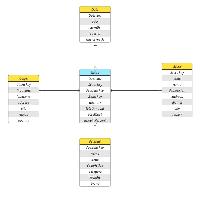
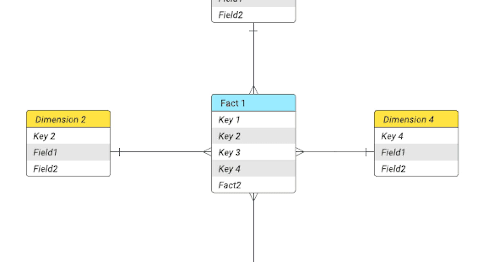
Is an arrangement of tables with the fact table in the center and the dimensions surrounding it, having a direct relationship with equal opportunities to contribute to the analysis of the fact table. The following diagram shows the shape of a star schema and how tables are arranged within it.

To better understand the properties of each table and its attributes, along with how the fact table relates to its dimensions, we provide an example of a sales fact table with its dimension and explain the properties of its components.

The provided example highlights the main characteristics of dimensions and fact table.

• Textual Attributes: Dimensions contain attributes with a descriptive nature such as product name, weight, and brand.

• Attributes not directly related: attributes in a dimension could not be related to each other such as the weight of a product and its brand name.

• Flat Dimensions, not normalized: In a star schema, dimensions are usually flat and contain all possible attributes without normalization. For example, if we were to normalize the customer dimension, we would have separate tables encapsulating the hierarchical relationships country — region — city in separate tables.

• Rolling up, Drilling down: The ability to look at data at different levels is what gives dimensional modeling its analytical power. In our example, we could aggregate the total quantities of a product listed in a country, but we could also break down the quantities within a region or a city.

• Data grain: Each row in the fact table tells us a little story a client buys a quantity of a specific product from a store located in a city at a date. so, this is the lowest granularity level, if we select the quantity by month the data granularity is at a higher level.

• The fact table and its different types of measures: The fact table contains metrics such as quantity sold, which is fully additive across all dimensions. If we assume that the percentage profit margin is the difference between the total amount and the total cost, this aggregation has no meaning if we add up the percentage profit margin for all customers in a city.

In essence, the Star schema is just a simple de-normalized relational model with one-to-many relationships. In the next part, we will highlight some of its advantages and disadvantages that make it the defacto structure for data warehouses.

Advantages:

• Simplicity: Star schema provides an intuitive design for users of the decision system by grouping all business metrics in the fact table and relating it to its business dimensions which gives us the ability to filter and analyze those metrics using the dimension's attributes.

• Optimize query processing and navigation: Each query starts with selecting rows from dimensions filtered by business criteria, then finding the corresponding rows in the fact table and finally applying aggregation operations.

Disadvantage:

• Slightly complex Extract-Transform-Load: a de-normalized dimension may require additional operations to populate data into it. This is done by joining tables in the source database to obtain descriptive attributes within the dimension.

Snowflake schema

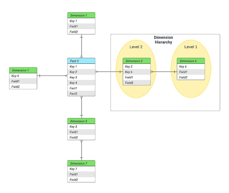
The idea behind the snowflake schema is to normalize dimension tables by encapsulating hierarchical levels in separate tables for all or only a few dimensions. In the star schema, we tend to flatten dimensions by integrating all hierarchical details into the dimension itself, resulting in a model in non-third form. Instead in Snowflake, we create a separate table with 1-to-many relationships.

In the next part, we will see some of the advantages and disadvantages of the snowflake schema and why the star schema is preferable to it as a denormalized schema.

Advantages:

• Small disk space optimization: snowflake optimizes storage space by not replicating de-normalized descriptive attributes throughout the dimension, such as the category name in the product dimension, since the text field would be small in size comparing it to a number key size.

• Simple to update: normalized structures are easy to update, only the order hierarchy has to be respected.

Disadvantage:

• Less intuitive navigation: When normalizing dimensions, the problem of navigating through hierarchies arises, leading to increased complexity for users to understand the structure and degradation in query performance for joins.

Constellation schema

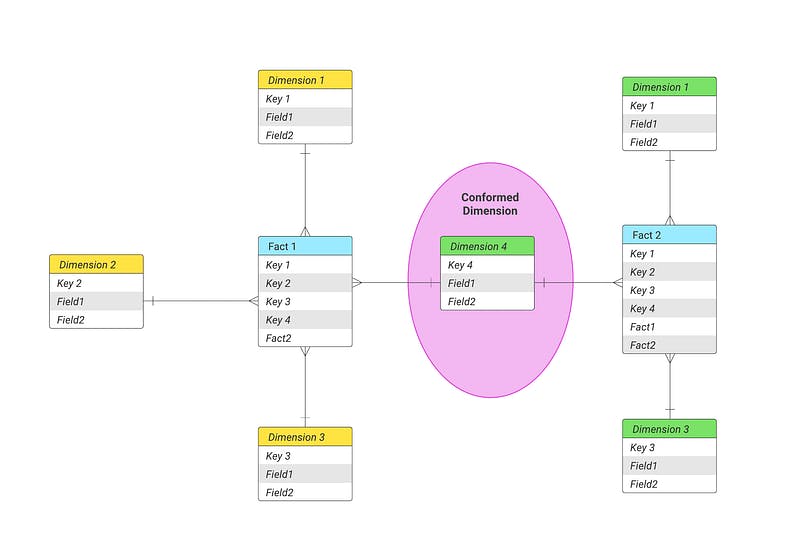
A connection between multiple star schema through dimensions or direct fact-to-fact relationship.

Throughout our blog, we have discussed various dimensional modeling techniques. In the next blog, we will see a mini case of how to transform an ERD model into a star schema. Stay tuned!